Stereo Vision Laboratory

11. Stereo Rectifier using Gaze_line-Depth Model

Z. Zhang's camera calibration method

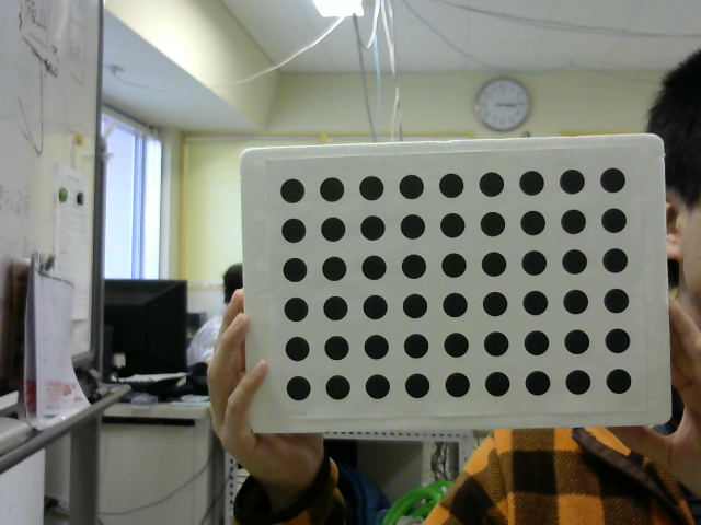
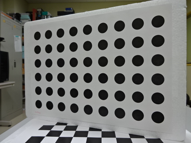
The well-known Z. Zhang technique ("A flexible new technique for camera calibration", IEEE Transactions on Pattern Analysis and Machine Intelligence, 22 (11): 1330-1334, 2000) uses an instrument such as

. Calibrate the camera. The focal length and distortion coefficient in units of camera pixels, and the position and orientation of the camera relative to the fixture from an image of the fixture with the feature points (center of the circle in the photo above) arranged in a grid on the plane I need it. Strangely, you don't need to know how many centimeters the distance between feature points is. When applied to a stereo camera, the positional relationship between the stereo cameras can also be understood. The OpenCV sample includes both single camera calibration and stereo camera calibration so you can try it out.

When you try it, it is difficult to obtain satisfactory results, and if you use two cheap USB cameras (Logitech C270 etc.) introduced in article 5, you can not get the stereo parallel accuracy that can be used for stereo vision did. I feel that the cause is that it is a rolling shutter and there is no simultaneousness because there are two USB connections in the first place. I think that the algorithm is weak for mathematically contradictory data. Researchers in the survey field have told me that it is linguistic, such as calibrating the camera with the calibration board in hand. However, it is not easy to fix to something because you have to shoot at various angles.

New camera calibration method

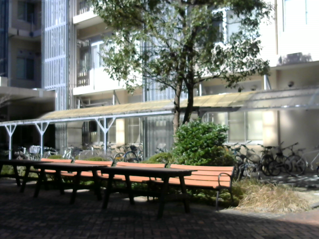
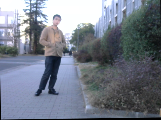
When I was thinking that there was no more robust method, I thought that the graph cut value of stereo vision by Gaze_line-Depth Model could be used for stereo rectification as it was, and I was a 4th year student at Oguri Lab. We set the theme for Toshizen Miyazaki's graduation research and proceeded together. At that time, Miyazaki-kun's photograph was approved and used on this page. First of all, look at the execution example to see what this method is called 3D Reconstruction Method.

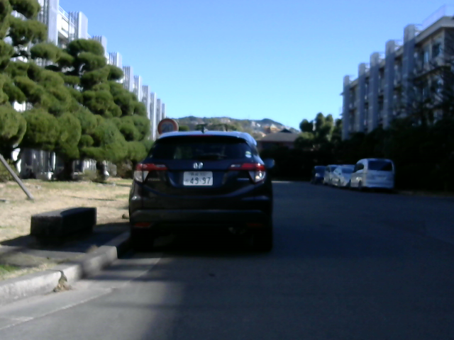
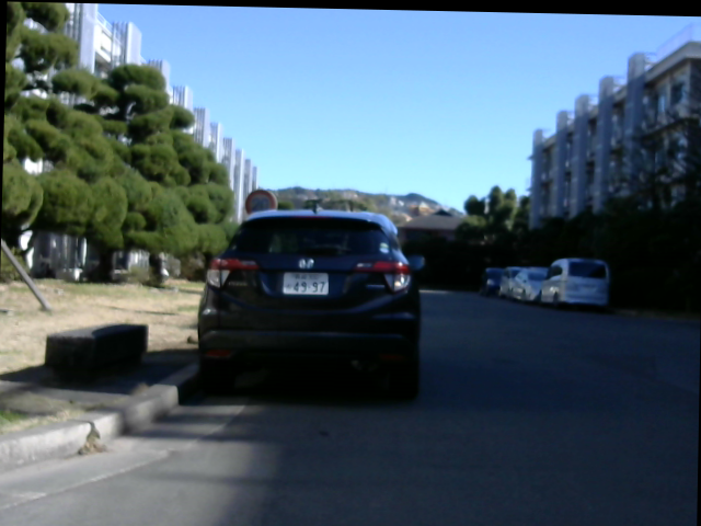
Stereo Rectifier execution example 1

First, right image display and left image display are repeated four times. If you look at this, you can see that it has rotated left and right. You can see how the parallelization process proceeds after this. The actual time is about the same as this video. When the parallel processing is completed, the right image display and the left image display are repeated four times. This time you can see that it is moving right next to it. The last is a 3D image restored from a stereo image that has been processed in parallel. The images before and after stereo parallelization are as follows.

In the following execution example, the left and right sides are greatly shifted, but they are parallelized properly.

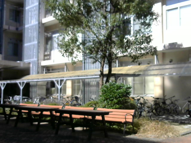
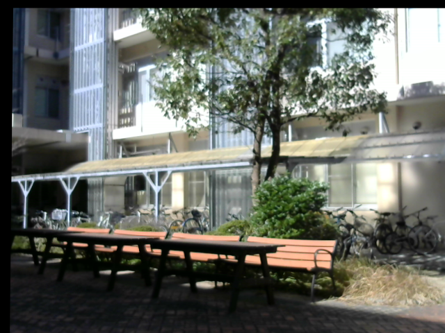
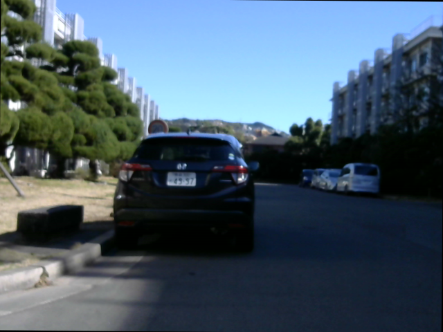
Stereo Rectifier execution example 2

The images before and after stereo parallelization are as follows.

The following execution example changes the distance continuously from near to far and there is almost no face-to-face, but this also works well.

Stereo Rectifier execution example 3

The images before and after stereo parallelization are as follows.

Principle of 3D reconstruction method

What I found in article 10 is that stereo parallelization can be achieved if the left and right camera images are properly rotated in three dimensions. Z.Zhang's method uses a priori calculation to calculate this rotation that can be stereo-parallelized. And since the calculation and order seem to be weak to data containing contradictions, let's consider a method that is as deductive as possible. In the first place, the fact that 3D is restored by minimizing the evaluation value of energy by graph cut means that the smaller the energy is, the more likely it is as 3D. It is thought that it can be judged by this energy. Therefore, repeat the process of adopting an arbitrary rotation to reduce the energy value for the three degrees of freedom of rotation with the left camera and three with the right camera, and stop when the energy no longer decreases I tried the basic method of doing this and it worked. There was no need to escape from the minimum.

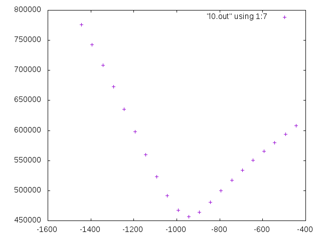
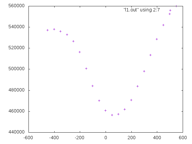
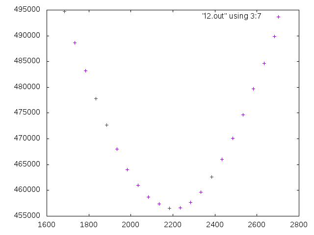
Examining how the energy changes around the convergence value of the rotation where it is no longer possible to reduce the energy compared to Example 1 above, it is

The rotation and convergence position of the left camera around the \(u\) axis is -944

The rotation and convergence position of the left camera around the \(v\) axis is 48

Rotation and convergence position around the optical axis of the left camera is 2184

The rotation and convergence position of the right camera around the \(u\) axis is 8

The rotation and convergence position of the right camera around the \(v\) axis is -40.

The rotation and convergence position around the optical axis of the right camera is 784

and a single-peak function form. You can see why stereo parallelization works well with simple processing.

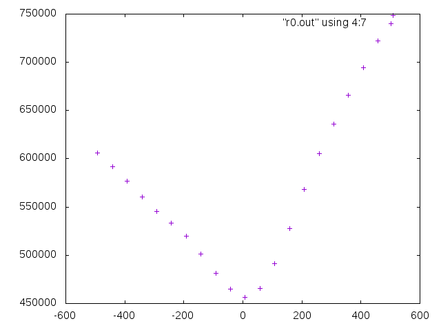
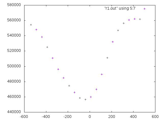
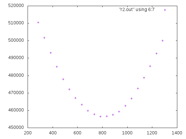
3D rotation of camera image

The 3D rotation of the camera image itself is performed using the OpenCV initUndistortRectifyMap function described in article 10, but before and after that, it looks like

void rotate(int l0, int l1, int l2, int r0, int r1, int r2) {
  cv::Mat M = cv::Mat::zeros(3, 3, CV_64F);
  M.at(0, 0) = focal/pixel;
  M.at(0, 2) = double(XX-1)/2;
  M.at(1, 1) = focal/pixel;
  M.at(1, 2) = double(YY-1)/2;
  M.at(2, 2) = 1.0;
  cv::Mat D = cv::Mat::zeros(1, 5, CV_64F);
  cv::Size S = cv::Size(XX, YY);
  cv::Mat lV = cv::Mat::zeros(1, 3, CV_64F);
  cv::Mat rV = cv::Mat::zeros(1, 3, CV_64F);
  lV.at(0, 0) = 0.00001*l0;
  lV.at(0, 1) = 0.00001*l1;
  lV.at(0, 2) = 0.00001*l2;
  rV.at(0, 0) = 0.00001*r0;
  rV.at(0, 1) = 0.00001*r1;
  rV.at(0, 2) = 0.00001*r2;
  cv::Mat lR;
  cv::Mat rR;
  Rodrigues(lV, lR);
  Rodrigues(rV, rR);
  cv::Mat lmap1;
  cv::Mat lmap2;
  cv::Mat rmap1;
  cv::Mat rmap2;
  initUndistortRectifyMap(M, D, lR, M, S, CV_16SC2, lmap1, lmap2);
  initUndistortRectifyMap(M, D, rR, M, S, CV_16SC2, rmap1, rmap2);
  remap(lframe, llframe, lmap1, lmap2, cv::INTER_LINEAR);
  remap(rframe, rrframe, rmap1, rmap2, cv::INTER_LINEAR);
}

. The six arguments of this rotate function are rotation around the \(u\) axis of the left image, rotation around the \(v\) axis, rotation around the optical axis, rotation around the \(u\) axis of the right image, rotation around the \(v\) axis, and rotation around the optical axis. It has become. The Rodrigues rotation vector is set from these and converted to a rotation matrix by the OpenCV Rodrigues function. Rodriguez's rotation vector has the meaning of rotating the vector by the magnitude of the vector, with the direction of the vector as the rotation axis. One rotation when the vector size is 2. In the caption of the previous graph, "-40" of "convergence position is -40" is the value of this argument. lframe and rframe are the original images and llframe and rrframe are the rotated images. The focal length of the camera matrix M was mentioned in article 10, but it is the focal length in pixels. Since the focal length is not known in the 3D reconstruction method described here, set the correct value. If it differs greatly from the correct value, it will not work.

Main body of 3D reconstruction method

The body of the 3D reconstruction method is

void calib(void) {
  int l0 = 0; int l1 = 0; int l2 = 0;
  int r0 = 0; int r1 = 0; int r2 = 0;
  rotate(l0, l1, l2, r0, r1, r2);
  int min = graph_cut();
  for (int mul = 512; mul >= 8; mul /= 2) {
    int flg = 0;
    int step = 0;
    for ( ; ; ) {
           if (step ==  0) l0+=mul; else if (step ==  1) r0-=mul;
      else if (step ==  2) l0-=mul; else if (step ==  3) r0+=mul;
      else if (step ==  4) l2+=mul; else if (step ==  5) r2-=mul;
      else if (step ==  6) l2-=mul; else if (step ==  7) r2+=mul;
      else if (step ==  8) l1+=mul; else if (step ==  9) r1-=mul;
      else if (step == 10) l1-=mul; else if (step == 11) r1+=mul;
      else {}
      rotate(l0, l1, l2, r0, r1, r2);
      int now = graph_cut();
      if (now >= min) {
             if (step ==  0) l0-=mul; else if (step ==  1) r0+=mul;
        else if (step ==  2) l0+=mul; else if (step ==  3) r0-=mul;
        else if (step ==  4) l2-=mul; else if (step ==  5) r2+=mul;
        else if (step ==  6) l2+=mul; else if (step ==  7) r2-=mul;
        else if (step ==  8) l1-=mul; else if (step ==  9) r1+=mul;
        else if (step == 10) l1+=mul; else if (step == 11) r1-=mul;
        else {}
      }
      else {
        flg = 1;
        min = now;
      }
      step++;
      if (step == 12) {
        if (flg == 0) break;
        flg = 0;
        step = 0;
      }
    }
  }
  rotate(l0, l1, l2, r0, r1, r2);
}

. The rotation trials are initially large and progressively smaller, but this is simply to reduce the number of trials.

Why the focal length can be determined by Z. Zhang's method

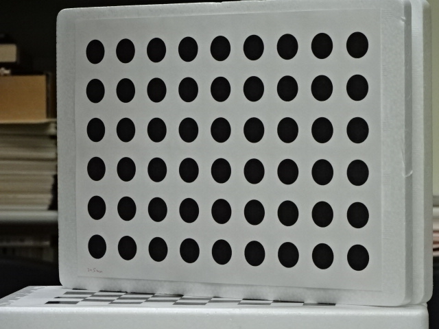
The next two pictures are the same calibration board taken with a camera with zoom function, that is, the focal length can be changed. Both are taken with the same tilt, and both have the calibration board on the right side and the left side on the back. In addition, the zoom was adjusted so that the right side on the near side was the same size in perspective. You can think of this size as a measure of length in pixels. The following lengths and distances are all relative to this standard. If you look at the vertical and horizontal intervals of a circle (ellipse?), You can see the inclination of the board and the depth distance (A). This is the same in the two cases. On the other hand, you can see the ratio (B) of the distance from the camera as it gets smaller as you go deeper. From the actual distance (A) and the distance ratio (B), the focal length in pixels is obtained.

Perspective calibration board (far left, far right)

If you apply the Z.Zhang method to a single tilted photo, rather than a dozen photos as in the OpenCV sample, you can stably determine the focal length of the camera. The focal length used in the 3D reconstruction method is the value obtained by the Z.Zhang method from a single tilted photograph. However, even if it is a little different, the results will not change that much.

Program distribution

graph_cut.cu Download rectify.cpp , makefile , 3_R.png , and 3_L.png .

make do

When you press and press the M key, you can see the stereo parallelization process in Example 1. The following one-character key commands can be used.

List of one character commands
character	function
q	quit
?	help
M	do calibration
m	left picture
,	stereo picture
.	right picture
<	both picture
s	depth(disparity) to front
t	depth(disparity) to back
h	eye move left angle
j	eye move down angle
k	eye move up angle
l	eye move right angle
f	eye move near
n	eye move far
H	eye move left
J	eye move down
K	eye move up
L	eye move right
F	eye move forward
N	eye move back
C	clear angle and position

The startup format is

./rec right_image left_image max_disparity min_disparity penalty inhibit divisor option

. For example, if the divisor value is 2, the graph will be cut with the vertical and horizontal depths halved. The execution example was created with a divisor value of 4. The option value is 0 or 1. If 1, the contents of the execution example will be output when the M key is pressed. When 0, only stereo parallelization is executed. graph_cut.cu has the same name as the previous article, but the return value is changed to the graph cut value.