3. Distribution of stereo vision program
I made a stereo vision program using graph cut. Use scene1.row3.col1.ppm , scene1.row3.col3.ppm and makefile as common files. scene1.row3.col1.ppm and scene1.row3.col3.ppm are the left and right images corresponding to the true value data in the TSUKUBA stereo image introduced in Article 2. When using GPU and CUDA, change the following make targets from dis_c to dis_g, dep_c to dep_g, and 3d_c to 3d_g. You are free to use all the programs distributed in this article (the MIT license).
Graph Cut Program for Stereo Vision
graph_cut.cpp And graph_cut.cu is the main body of the graph cut program. graph_cut.cpp is a graph cut by CPU, and graph_cut.cu is a graph cut by GPU. In both cases, graph cut is performed on 3D Grid Graph by Push Relabel + Global Update method. The Global Update part uses a queue algorithm on the CPU and a shared memory algorithm on the GPU. These are completely different algorithms. On the other hand, the Push Relabel part uses the same algorithm for CPU and GPU.
Graph cut is performed by setting the global variable
- int SIZE_S;
- int SIZE_H;
- int SIZE_W;
- int SIZE_HW;
- int SIZE_SHW;
The 3D Grid Graph that is the target of the graph cut is a 10-adjacent branch graph dedicated to stereo vision as shown in the following figure.
However, the figure shows only the depth direction S and the horizontal direction W, and the vertical direction H is not visible.
The direction from the source node S to the sink node T is called the depth direction.
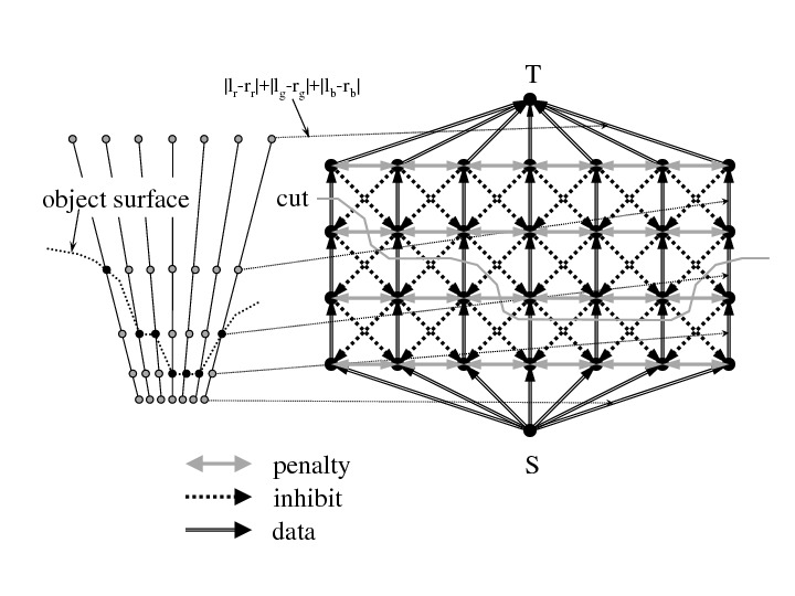
- 0: (reverse=9) (init_val=data_cost) front
- 1: (reverse=2) (init_val=penalty_h) up
- 2: (reverse=1) (init_val=penalty_h) down
- 3: (reverse=4) (init_val=penalty_w) left
- 4: (reverse=3) (init_val=penalty_w) right
- 5: (reverse=7) (init_val=zero) front right
- 6: (reverse=8) (init_val=zero) front left
- 7: (reverse=5) (init_val=inhibit_b) back left
- 8: (reverse=6) (init_val=inhibit_b) back right
- 9: (reverse=0) (init_val=inhibit_a) back
The size of the 3D Grid Graph is given by the global variable
- int SIZE_S;
- int SIZE_H;
- int SIZE_W;
In the true parallax image of the TSUKUBA stereo benchmark introduced in Article 2, the maximum parallax (max_disparity) is 28 and the minimum parallax (min_disparity) is 10, so if SIZE_S = max_disparity -min_disparity = 18, there are 19 labels from 0 to 18 You This corresponds to 10 to 28. In this way, SIZE_S itself is the number of nodes, but when viewed as a label, it represents the maximum label and the minimum label is 0, so the number of labels is SIZE_S +1. You should be aware of this whenever you are creating a program.
Pixel-Disparith Model
disparity_stereo.cpp Is a program that generates parallax image files by pixel-disparity model.
make dis_c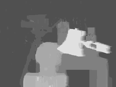
The pixel-disparity model can be seen from the cost () function
int cost(int D, int H, int W) {
  D += Min_depth;
  int RR, RG, RB;
  int LR, LG, LB;
  int LW;
  if (W+D > SIZE_W-1) LW = SIZE_W-1;
  else                LW = W+D;
  call_rgb(rframe, H, W, &RR, &RG, &RB);
  call_rgb(lframe, H, LW, &LR, &LG, &LB);
  int d_R = (LR>RR)? LR-RR: RR-LR;
  int d_G = (LG>RG)? LG-RG: RG-LG;
  int d_B = (LB>RB)? LB-RB: RB-LB;
  return d_R + d_G + d_B;
}Execution is
./disparity_cpu right_image left_image max_disparity min_disparity penalty inhibit sacleGaze_line-Depth Model
depth_stereo.cpp Is a program that generates parallax image files by gaze_line-depth model.
make dep_c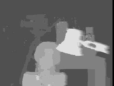
The gaze_line-depth model is the cost () function
int cost(int D, int H, int W) {
  D += Min_depth;
  int RR, RG, RB;
  int LR, LG, LB;
  int RW;
  int LW;
  if ((W-D < 0) && (W+D > SIZE_W-1)) {
    printf("Error\n");
  }
  else if (W-D < 0) {
    RW = 0;
    LW = 2*W;
  }
  else if (W+D > SIZE_W-1) {
    LW = SIZE_W-1;
    RW = SIZE_W-1-2*(SIZE_W-1-W);
  }
  else {
    RW = W-D;
    LW = W+D;
  }
  call_rgb(rframe, H, RW, &RR, &RG, &RB);
  call_rgb(lframe, H, LW, &LR, &LG, &LB);
  int d_R = (LR>RR)? LR-RR: RR-LR;
  int d_G = (LG>RG)? LG-RG: RG-LG;
  int d_B = (LB>RB)? LB-RB: RB-LB;
  return d_R + d_G + d_B;
}Execution is
./depth_cpu right_image left_image max_disparity min_disparity penalty inhibit magnification scale3D Stereo Vision Program
3d_stereo.cpp Is a program that displays the result of stereo vision processing by gaze_line-depth model in 3D.
make 3d_c| character | function |
|---|---|
| q | quit |
| ? | help |
| e | toggle figure mode |
| m | left picture |
| , | stereo picture (do graph_cut) |
| . | right picture |
| s | depth(disparity) to front |
| t | depth(disparity) to back |
| h | eye move left |
| j | eye move down |
| k | eye move up |
| l | eye move right |
| f | eye move far |
| n | eye move near |
| ! | decrease base line |
| @ | increase base line |
| # | decrease focal length |
| $ | ncrease focal length |
| % | decrease pixel size |
| ^ | increase pixel size |
| z | decrease penalty |
| x | increase penalty |
| Z | decrease inhibit |
| X | increase inhibit |
The program starts with
./3d_cpu right_image left_image max_disparity min_disparity penalty inhibit magnificationBackground knowledge
Stereo matching is a technique that detects the difference between the corresponding points in the left and right images, that is, the parallax, and estimates the spatial arrangement of the target from this parallax. Estimating the spatial position from the parallax is only triangulation, so it has been considered that the essence of the problem is how to find the corresponding point. Therefore, the problem of estimating the spatial position from left and right stereo images is called stereo matching. Textbook chapters and item names are usually not stereo vision but stereo matching. After 2D (image) processing to find corresponding points from two images, 3D processing to determine the arrangement of the space is performed, that is, it has been treated as separate processing. The purpose of this HP is to rethink stereovision, which has been too constrained by the term stereo matching and the concept of parallax to try to find correspondence, but for the time being I will explain the way of thinking so far.
In order to find correspondences, similarity of feature quantities and feature correspondence detection of featured points (called feature points and corners), similarity of images in rectangular areas, etc. have been used. These were classified as
- Feature-based stereo matching
- Region-based stereo matching
- Pixel-based stereo matching
Dense stereo solves the problem of assigning parallax to every pixel in the right image. The reason for assigning parallax to the right image is that it is natural to set the right direction to be positive, so if the parallax is positive, the point on the space projected on a pixel in the right image is slightly Since it is projected onto the pixel, it is natural that the right image in the left image is called parallax, and "right parallax, that is, positive parallax is assigned to the pixel in the right image".
The problem of assigning parallax to all pixels in the right image is called the site labeling problem. The site is a matter of assigning some label to a place because of the place. In this case, pixels are places and parallax is labels. The number of allocations is a huge number of labels, \begin{align*} assign\_num=label\_num^{site\_num} .\end{align*} Of these, one assignment is selected. Usually, a function that gives a single numerical value for the assignment is defined, and the assignment that minimizes the numerical value is selected. I feel that it's OK to judge whether a single number is good or bad, but this is an analogy from physics, and a function that gives a single real value of energy (such a function is called a Hamiltonian) It mimics the formulation of knowing all the systems. Therefore, this single numerical value assigned to the assignment is called energy, the function that gives energy is called the energy function, and choosing the smallest one is called energy minimization. Allocation is sometimes referred to as placement, a term used to describe physical states.
The energy function of the site labeling problem is expressed as \begin{align*} E(f)=E_{data}(f)+E_{smooth}(f) \end{align*} with \(f\) assigned. For simplicity, the site will be described as pixels and the label as parallax. First, \(E_{data}(f)\) is a term that determines whether the parallax assignment is appropriate for each pixel from the image data. This term alone is sufficient for stereo images where the correspondence is clearly seen by looking at only the pixels, but since only pixels of the same brightness and color are actually used, the second term \(E_{smooth}(f)\) looks at the relationship between the pixels. will become necessary. How to do this second term is a very important issue and various things have been proposed. The first step is to start with two adjacent pixels. For example, the parallax will usually not change that much between adjacent pixels. In other words, the second term is about smoothness, so the name \(E_{smooth}\) is used.
The case where the relationship between two sites is a problem is called the first floor, and the case where the relationship between three or more sites is a problem is called a higher floor. It is a big problem how to make a function even on the first floor. In particular, parallax changes smoothly for the most part, but naturally changes greatly at the boundary of the object, so it has been considered a troublesome thing that should not be simply made smooth. Therefore, a function called truncated linear is often used, which increases the energy according to the change for a small change, but does not increase the energy beyond a certain level. Increasing the energy of a certain arrangement corresponds to making it difficult for such an arrangement to occur. On the other hand, the depth in the gaze_line-depth model does not change greatly at the boundary of the object as in the case of disparity, so a simple proportional function can be used. Actually, there is a prohibition condition, so the depth can only change by a maximum of 1 between neighbors. It can be a convex function with forbidden conditions.
Also, it is strongly dependent on the shape of the energy function whether it is easy to find an arrangement that minimizes energy. When the energy function on the first floor has a property called convex, the minimum arrangement can be obtained at once using graph cut. Because truncated linear is not convex, approximation algorithms such as alpha expansion and alpha-beta swap are used.
The first disparity_stereo.cpp introduced in this article uses the linear energy function to find the minimum arrangement of pixel-disparity model at once. This linear energy function is expressed as \(E_{smooth}(f)=penalty*|i-j|\) for a site pair. Here, \(i\) and \(j\) are disparity values of adjacent pixels.
The second depth_stereo.cpp and the third 3d_stereo.cpp use the convex energy function to find the minimum arrangement at a stretch using the gaze_line depth model. This convex energy function is expressed as \begin{align*} E_{smooth}(f)=penalty*|i-j|+inhibit*(|i-j|-1)*T(|i-j|>1) \end{align*} for the site pair. Where \(i\) and \(j\) are the depth values of adjacent gaze_lines. \(T(bool)\) is a delta function that is 1 when \(bool\) is true and 0 otherwise. As you can see from this equation, increasing the inhibit will change the depth value of the adjacent gaze_line by only 1 at maximum. This inhibit has realized the important property of the gaze_line-depth model pointed out in Article 2. This makes it possible to use a convex energy function that can be completely minimized by graph cut, without having to consider the troublesome parallax property of changing smoothly at the boundary of the object, although it changes smoothly at most. It became.